Although lidars used to be the most expensive components of self-driving cars, and could easily cost you as much as $75,000 just a couple of years ago, prices have plummeted recently and there are really good lidar sensors on the market in sub-$8000 range these days. And it just keeps getting better as Velodyne has just announced a whole magnitude cheaper model range with a limited field-of-view, presumably costing just under $1000.

Dataset

Luckily, you don’t have to spend that much money to get hold of data generated by a lidar. KITTI Vision Benchmark Suite contains datasets collected with a car driving around rural areas of a city — a car equipped with a lidar and a bunch of cameras, of course. Some of those datasets are labeled, e.g. they also contain information about objects around it; we will visualize those as well. These datasets are publicly available here, if you would like to follow along just go ahead and download one of them.

I will use the 2011_09_26_drive_0001 dataset and corresponding tracklets, e.g. labeled surrounding objects. It is one of the smallest datasets out there (0.4 GB) which contains data for just 11 seconds of driving:

• Length: 114 frames (00:11 minutes)
• Image resolution: 1392 x 512 pixels
• Labels: 12 Cars, 0 Vans, 0 Trucks, 0 Pedestrians, 0 Sitters, 2 Cyclists, 1 Trams, 0 Misc

Dependencies

A lidar operates by streaming a laser beam at high frequencies, generating a 3D point cloud as an output in realtime. We are going to use a couple of dependencies to work with the point cloud presented in the KITTI dataset: apart from the familiar toolset of numpy and matplotlib we will use pykitti. In order to make tracklets parsing math easier we will use a couple of methods originally implemented by Christian Herdtweck that I have updated for Python 3, you can find them in source/parseTrackletXML.py in the project repo.

Visualization

Cameras

In addition to the lidar 3D point cloud data KITTI dataset also contains video frames from a set of forward facing cameras mounted on the vehicle. The regular camera data is not half as exciting as the lidar data, but is still worth checking out.

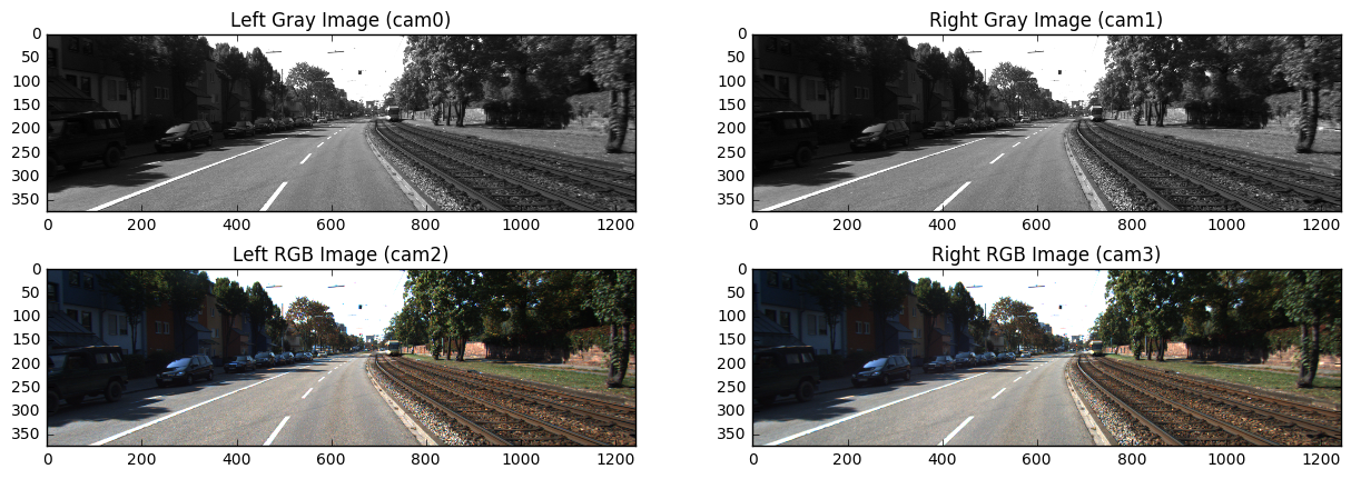Sample frames from cameras

Camera frames look pretty straightforward: you can see a tram track on the right with a lonely tram far ahead and some parked cars on the left. Although those road features may seem obvious to detect to you, a computer vision algorithm would struggle to differentiate those by relying solely on the visual data.

Lidar

The dataset in question contains 114 lidar point cloud frames over duration of 11 seconds. This equals to approximately 10 frames per second, which is a very decent scanning rate, given that we get a 360° field-of-view with each frame containing approximately 120,000 points — a fair amount of data to stream in realtime. Not to clutter the visualizations we will randomly sample 20% of the points for each frame and discard the rest.

We will additionally visualize tracklets, e.g. labeled objects like cars, trams, pedestrians and so on. With a bit of math we will grab information from the KITTI tracklets file and work out each object’s bounding box for each frame, feel free to check out the notebook for more details. There are only 3 types of objects in this particular 11-seconds piece, we will mark them with bounding boxes as follows: cars will be marked in blue, trams in red and cyclists in green. Let’s first visualize a sample lidar frame on a 3D plot.

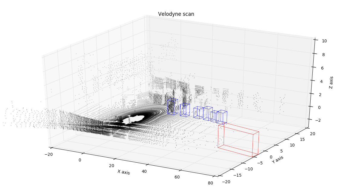Sample lidar frame

Looks pretty neat! You can see the car with a lidar in the center of a black circle, with laser beams coming out of it. You can even see silhouettes of the cars parked on the left side of the road and tram tracks on the right! And of course bounding boxes for tram and cars, they seem to be exactly where you would expect them looking at the regular camera data. You might have also noticed that only the objects that are visible to the cameras are labeled.

Having this data as a point cloud is extremely useful, as it can be represented in various ways specific to particular applications. You could scale the data points over some particular axis, or simply discard one of the axes to create a plane projection of the point cloud. This is what this velodyne frame would look like when projected on XZ, XY and YZ planes respectively:

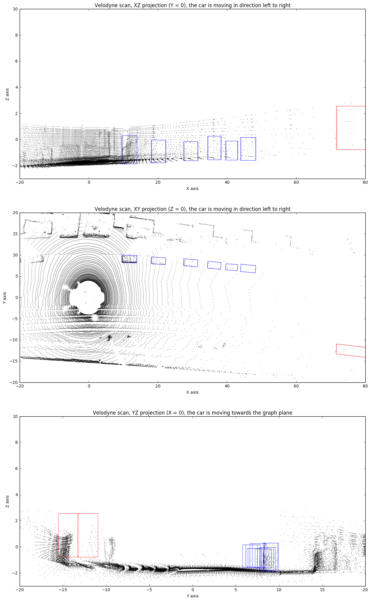Projections of a sample lidar frame

Usually you can significantly improve your model performance by preprocessing the data. What you are trying to achieve is a reduction in dimensionality of the input, hoping to extract some useful features and remove those that would be redundant or slow down and confuse the model. In this particular case discarding Z coordinate seems like a promising path to explore, as it gives us pretty much a bird’s-eye view of the vehicle surroundings. With a more sophisticated feature-engineering coupled with regular camera data as an additional input, you could achieve decent performance on detecting and classifying surrounding objects.

Finally, let’s plot all 114 sequential frames and combine them into a short video representing how point cloud changes over time.

Lidar data plotted over time

This should give a much better idea of what lidar data looks like. You can clearly see silhouettes of trees and parked cars that our vehicle is passing by — now that would be much easier for an algorithm to interpret. And although lidar is usually used in conjunction with a bunch of other sensors and data sources, it plays a significant role in vehicle simultaneous localization and mapping.

Follow @alexstaravoitau Star Fork Download