We are going to try detecting and tracking some basic road features in a video stream from a front-facing camera on a vehicle, this is clearly a very naive way of doing it and can hardly be applied in the field, however it is a good representation of what we can detect using mainly computer vision techniques: e.g. fiddling with color spaces and various filters. We will cover tracking of the following features:

• Lane boundaries. Understanding where the lane is could be useful in many applications, be it a self-driving car or some driving assistant software.
• Surrounding vehicles. Keeping track of other vehicles around you is just as important if you were to implement some collision-avoiding algorithm.

We will implement it in two major steps, first we will prepare a pipeline for lane tracking, and will then learn how to detect surrounding vehicles.

Road features detection is one of the assignments in Udacity Self-Driving Car Nanodegree program, however the concepts described here should be easy to follow even without that context.

Source video

I am going to use a short video clip shot from a vehicle front-facing camera while driving on a highway. It was shot in close to perfect conditions: sunny weather, not many vehicles around, road markings clearly visible, etc. — so using just computer vision techinques alone should be sufficient for a quick demonstration. You can check out the full 50 seconds video here.

Source video

Lane Tracking

Let’s first prepare a processing pipeline to identify the lane boundaries in a video. The pipeline includes the following steps that we apply to each frame:

• Camera calibration. To cater for inevitable camera distortions, we calculate camera calibration using a set of calibration chessboard images, and applying correction to each of the frames.
• Edge detection with gradient and color thresholds. We then use a bunch of metrics based on gradients and color information to highlight edges in the frame.
• Perspective transformation. To make lane boundaries extraction easier we apply a perspective transformation, resulting in something similar to a bird’s eye view of the road ahead of the vehicle.
• Fitting boundary lines. We then scan resulting frame for pixels that could belong to lane boundaries and try to approximate lines into those pixels.
• Approximate road properties and vehicle position. We also provide a rough estimate on road curvature and vehicle position within the lane using known road dimensions.

Camera calibration

We are going to use some heavy image warping on later stages, which would make any distortions introduced by the camera lense very apparent. So in order to cater for that we will introduce a camera correction step based on a set of calibration images shot with the same camera. A very common techinque would be shooting a printed chessboard from various angles and calculating the distortions introduced by the camera based on the expected chessboard orientation in the photo.

We are going to use a number of OpenCV routines in order to apply correction for camera distortion. I first prepare a pattern variable holding object points in (x, y, z) coordinate space of the chessboard, which are essentially inner corners of the chessboard. Here x and y are horizontal and vertical indices of the chessboard squares, and z is always 0 (as chessboard inner corners lie in the same plane). Those object points are going to be the same for each calibration image, as we expect the same chessboard in each.

pattern = np.zeros((pattern_size[1] * pattern_size[0], 3), np.float32)
pattern[:, :2] = np.mgrid[0:pattern_size[0], 0:pattern_size[1]].T.reshape(-1, 2)

We then use cv2.findChessboardCorners() function to get coordinates of the corresponding corners in each calibration image.

pattern_points = []
image_points = []
found, corners = cv2.findChessboardCorners(image, (9, 6), None)
if found:
    pattern_points.append(pattern)
    image_points.append(corners)

Once we have collected all the points from each image, we can compute the camera calibration matrix and distortion coefficients using the cv2.calibrateCamera() function.

_, self.camera_matrix, self.dist_coefficients, _, _ = cv2.calibrateCamera(
    pattern_points, image_points, (image.shape[1], image.shape[0]), None, None
)

Now that we have camera calibration matrix and distortion coefficients we can use cv2.undistort() to apply camera distortion correction to any image.

corrected_image = cv2.undistort(image, self.camera_matrix, self.dist_coefficients, None, self.camera_matrix)

As some of the calibration images did not have chessboard fully visible, we will use one of those for verifying aforementioned calibration pipeline.

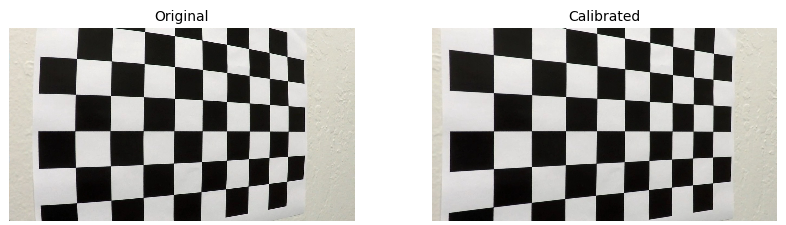Original vs. calibrated images

For implementation details check CameraCalibration class in lanetracker/camera.py.

Edge detection

We use a set of gradient and color based thresholds to detect edges in the frame. For gradients we use Sobel operator, which essentially highlights rapid changes in color over either of two axes by approximating derivatives using a simple convolution kernel. For color we simply convert the frame to HLS color space and apply a threshold on the S channel. The reason we use HLS here is because it proved to perform best in separating light pixels (road markings) from dark pixels (road) using the saturation channel.

• Gradient absolute value. For absolute gradient value we simply apply a threshold to `cv2.Sobel() output for each axis.

sobel = np.absolute(cv2.Sobel(image, cv2.CV_64F, 1, 0, ksize=3))

• Gradient magnitude. Additionaly we include pixels within a threshold of the gradient magnitude.

sobel_x = cv2.Sobel(image, cv2.CV_64F, 1, 0, ksize=3)
sobel_y = cv2.Sobel(image, cv2.CV_64F, 0, 1, ksize=3)
magnitude = np.sqrt(sobel_x ** 2 + sobel_y ** 2)

• Gradient direction. We also include pixels that happen to be withing a threshold of the gradient direction.

sobel_x = cv2.Sobel(image, cv2.CV_64F, 1, 0, ksize=3)
sobel_y = cv2.Sobel(image, cv2.CV_64F, 0, 1, ksize=3)
direction = np.arctan2(np.absolute(sobel_y), np.absolute(sobel_x))

• Color. Finally, we extract S channel of image representation in the HLS color space and then apply a threshold to its absolute value.

hls = cv2.cvtColor(np.copy(image), cv2.COLOR_RGB2HLS).astype(np.float)
s_channel = hls[:, :, 2]

We apply a combination of all these filters as an edge detection pipeline. Here is an example of its output, where pixels masked by color are blue, and pixels masked by gradient are green.

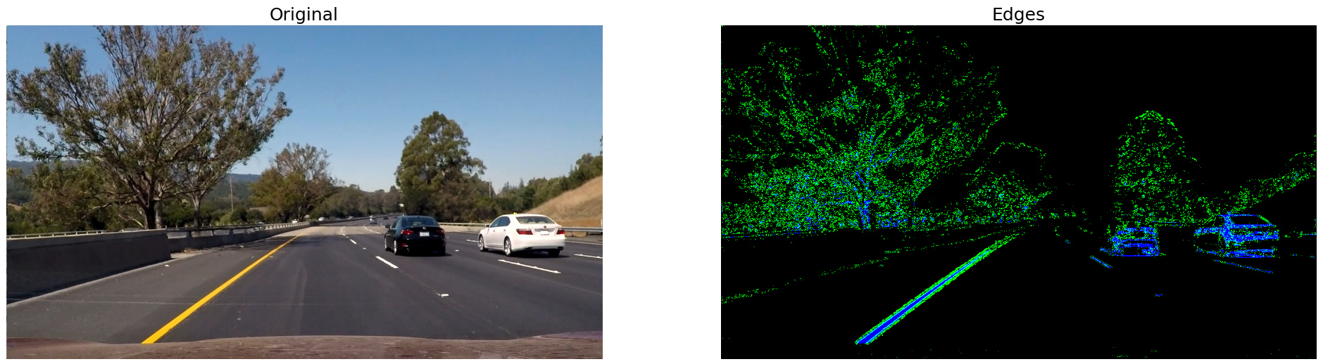
Original vs. highlighted edges

For implementation details check functions in lanetracker/gradients.py.

Perspective transform

It would be much easier to detect lane boundaries if we could get hold of a bird’s eye view of the road, and we can get something fairly close to it by applying a perspective transform to the camera frames. For the sake of this demo project I manually pin-pointed source and destination points in the camera frames, so perspective transform simply maps the following coordinates.

The transformation is applied using cv2.getPerspectiveTransform() function.

(h, w) = (image.shape[0], image.shape[1])
source = np.float32([[w // 2 - 76, h * .625], [w // 2 + 76, h * .625], [-100, h], [w + 100, h]])
destination = np.float32([[100, 0], [w - 100, 0], [100, h], [w - 100, h]])
transform_matrix = cv2.getPerspectiveTransform(source, destination)
image = cv2.warpPerspective(image, transform_matrix, (w, h))

This is what it looks like for an arbitrary test image.

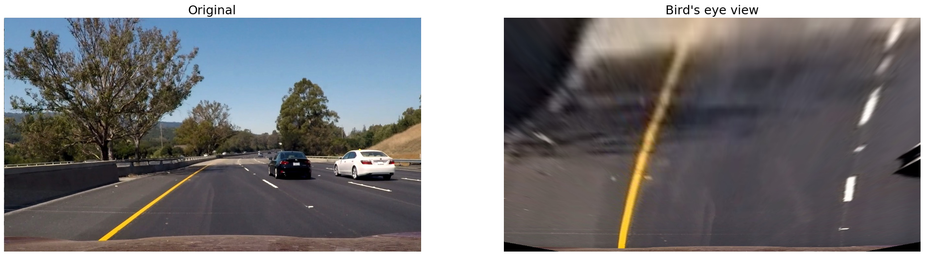
Original vs. bird’s eye view

For implementation details check functions in lanetracker/perspective.py.

Detect boundaries

We are now going to scan the resulting frame from bottom to top trying to isolate pixels that could be representing lane boundaries. What we are trying to detect is two lines (each represented by Line class) that would make up lane boundaries. For each of those lines we have a set of windows (represented by Window class). We scan the frame with those windows, collecting non-zero pixels within window bounds. Once we reach the top, we try to fit a second order polynomial into collected points. This polynomial coefficients would represent a single lane boundary.

Here is a debug image representing the process. On the left is the original image after we apply camera calibration and perspective transform. On the right is the same image, but with edges highlighted in green and blue, scanning windows boundaries highlighted in yellow, and a second order polynomial approximation of collected points in red.

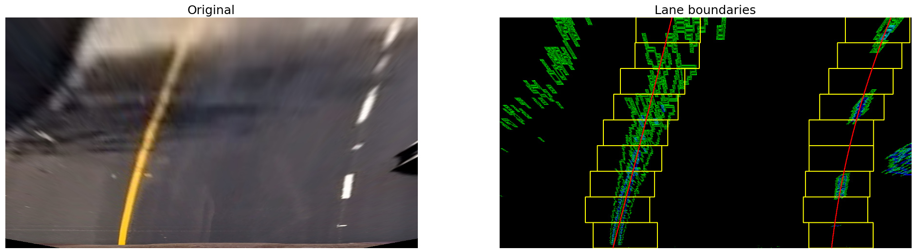
Boundary detection pipeline

For implementation details check LaneTracker class in lanetracker/tracker.py, Window class in lanetracker/window.py and Line class in lanetracker/line.py.

Approximate properties

We can now approximate some of the road properties and vehicle spacial position using known real world dimensions. Here we assume that the visible vertical part of the bird’s eye view warped frame is 27 meters, based on the known length of the dashed lines on american roads. We also assume that lane width is around 3.7 meters, again, based on american regulations.

ym_per_pix = 27 / 720  # meters per pixel in y dimension
xm_per_pix = 3.7 / 700  # meters per pixel in x dimension

Road curvature

Previously we approximated each lane boundary as a second order polynomial curve, which can be represented with the following equation.

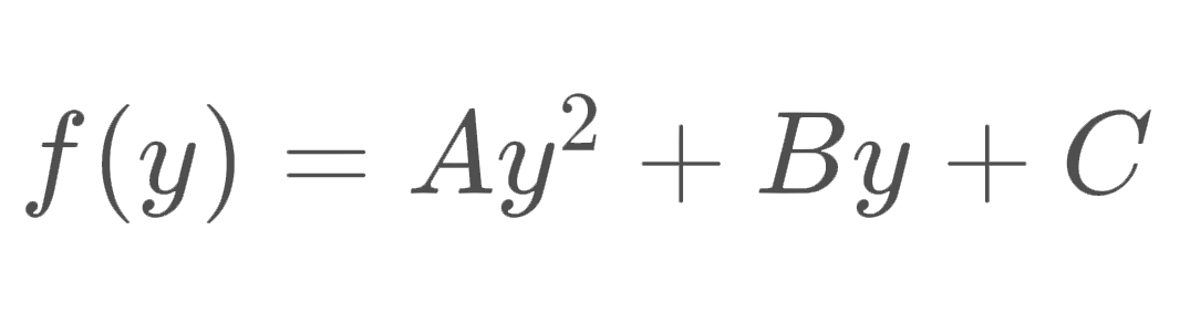Second order polynomial

As per this tutorial, we can get the radius of curvature in an arbitrary point using the following equation.

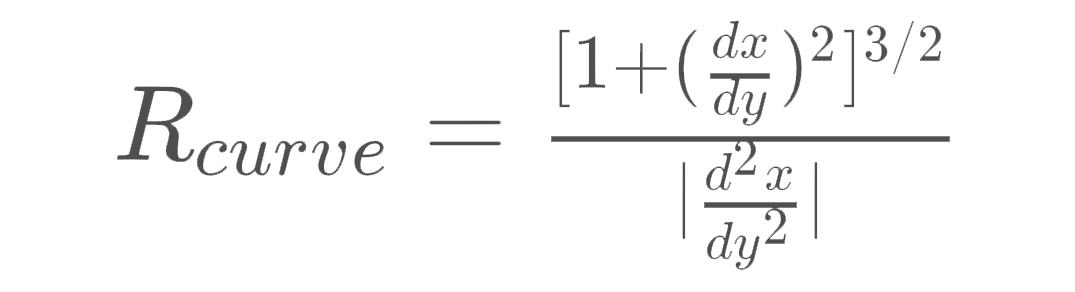Radius equation

If we calculate actual derivatives of the second order polynomial, we get the following.

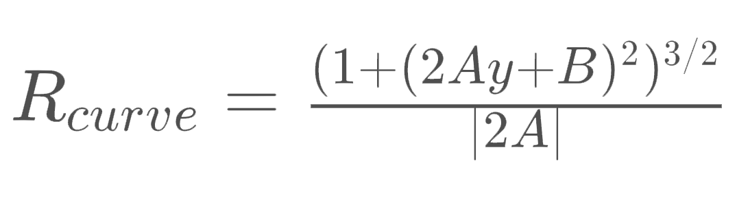Radius equation

Therefore, given x and y variables contain coordinates of points making up the curve, we can get curvature radius as follows.

# Fit a new polynomial in real world coordinate space
poly_coef = np.polyfit(y * ym_per_pix, x * xm_per_pix, 2)
radius = ((1 + (2 * poly_coef[0] * 720 * ym_per_pix + poly_coef[1]) ** 2) ** 1.5) / np.absolute(2 * poly_coef[0])

Vehicle position

We can also approximate vehicle position within the lane. This rountine would calculate an approximate distance to a curve at the bottom of the frame, given that x and y contain coordinates of points making up the curve.

(h, w, _) = frame.shape
distance = np.absolute((w // 2 - x[np.max(y)]) * xm_per_pix)

For implementation details check Line class in lanetracker/line.py.

Sequence of frames

We can now try to apply the whole pipeline to a sequence of frames. We will use an approximation of lane boundaries detected over last 5 frames in the video using a deque collection type. It will make sure we only store last 5 boundary approximations.

from collections import deque

coefficients = deque(maxlen=5)

We then check if we detected enough points (x and y arrays of coordinates) in the current frame to approximate a line, and append polynomial coefficients to coefficients. The sanity check here is to ensure detected points span over image height, otherwise we wouldn’t be able to get a reasonable line approximation.

if np.max(y) - np.min(y) > h * .625:
    coefficients.append(np.polyfit(y, x, 2))

Whenever we want to draw a line, we get an average of polynomial coefficients detected over last 5 frames.

mean_coefficients = np.array(coefficients).mean(axis=0)

This approach proved iself to work reasonably well, you can check out the full annotated video here.

Sample of the annotated project video

For implementation details check LaneTracker class in lanetracker/tracker.py.

Vehicle Tracking

We are going to use a bit of machine learning to detect vehicle presence in an image by training a classifer that would classify an image as either containing or not containing a vehicle. We will train this classifer using a dataset provided by Udacity which comes in two separate archives: images containing cars and images not containing cars. The dataset contains 17,760 color RGB images 64×64 px each, with 8,792 samples labeled as containing vehicles and 8,968 samples labeled as non-vehicles.

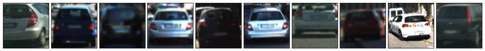Random sample labeled as containing cars

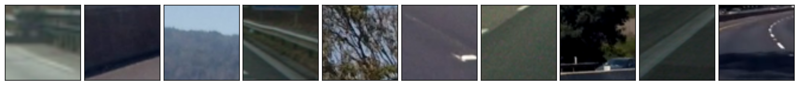Random sample of non-cars

In order to prepare a processing pipeline to identify surrounding vehicles, we are going to break it down into the following steps:

• Extract features and train a classifier. We need to identify features that would be useful for vehicle detections and prepare a feature extraction pipeline. We then use it to train a classifier to detect a car in individual frame segment.
• Apply frame segmentation. We then segment frame into windows of various size that we run through the aforementioned classifier.
• Merge individual segment detections. As there will inevitably be multiple detections we merge them together using a heat map, which should also help reducing the number of false positives.

Feature extraction

After experimenting with various features I settled on a combination of HOG (Histogram of Oriented Gradients), spatial information and color channel histograms, all using YCbCr color space. Feature extraction is implemented as a context-preserving class (FeatureExtractor) to allow some pre-calculations for each frame. As some features take a lot of time to compute (looking at you, HOG), we only do that once for entire image and then return regions of it.

Histogram of Oriented Gradients

I had to run a bunch of experiments to come up with final parameters, and eventually I settled on HOG with 10 orientations, 8 pixels per cell and 2 cells per block. The experiments went as follows:

1. Train and evaluate the classifier for a wide range of parameters and identify promising smaller ranges.
2. Train and evaluate the classifier on those smaller ranges of parameters multiple times for each experiment and assess average accuracy.

The winning combination turned out to be the following:

 orient     px/cell    clls/blck  feat-s     iter       acc        sec/test  
 10         8          2          5880       0          0.982      0.01408   
 10         8          2          5880       1          0.9854     0.01405   
 10         8          2          5880       2          0.9834     0.01415   
 10         8          2          5880       3          0.9825     0.01412   
 10         8          2          5880       4          0.9834     0.01413   
Average accuracy = 0.98334

This is what Histogram of Oriented Gradients looks like applied to a random dataset sample.

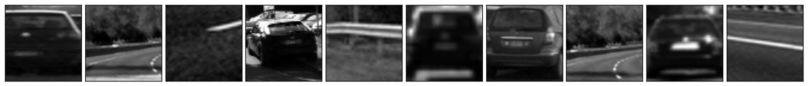Original (Y channel of YCbCr color space)

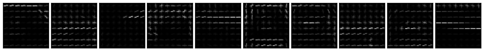HOG (Histogram of Oriented Gradients)

Initial calculation of HOG for entire image is done using hog() function in skimage.feature module. We concatenate HOG features for all color channels.

(h, w, d) = image.shape
hog_features = []
for channel in range(d):
    hog_features.append(
        hog(
            image[:, :, channel], 
            orientations=10, 
            pixels_per_cell=(8, 8),
            cells_per_block=(2, 2), 
            transform_sqrt=True,
            visualise=False, 
            feature_vector=False
        )
    )
hog_features = np.asarray(hog_features)

This allows us to get features for an individual image window by calculating HOG array offsets, given that x is the window horizontal offset, y is the vertical offset and k is the size of the window (single value, side of a square region).

hog_k = (k // 8) - 1
hog_x = max((x // 8) - 1, 0)
hog_x = hog_features.shape[2] - hog_k if hog_x + hog_k > hog_features.shape[2] else hog_x
hog_y = max((y // 8) - 1, 0)
hog_y = hog_features.shape[1] - hog_k if hog_y + hog_k > hog_features.shape[1] else hog_y
region_hog = np.ravel(hog_features[:, hog_y:hog_y+hog_k, hog_x:hog_x+hog_k, :, :, :])

Spatial information

For spatial information we simply resize the image to 16×16 and flatten to a 1-D vector.

spatial = cv2.resize(image, (16, 16)).ravel()

Color channel histogram

We additionally use individual color channel histogram information, breaking it into 16 bins within (0, 256) range.

color_hist = np.concatenate((
    np.histogram(image[:, :, 0], bins=16, range=(0, 256))[0],
    np.histogram(image[:, :, 1], bins=16, range=(0, 256))[0],
    np.histogram(image[:, :, 2], bins=16, range=(0, 256))[0]
))

FeatureExtractor

The way FeatureExtractor class works is that you initialise it with a single frame, and then request a feature vector for individual regions. In this case it only calculates computationally expensive features once. You then call feature_vector() method to get a concatenated combination of HOG, spatial and color histogram feature vectors.

extractor = FeatureExtractor(frame)

# Feature vector for entire frame
feature_vector = extractor.feature_vector()

# Feature vector for a 64×64 frame region at (0, 0) point
feature_vector = extractor.feature_vector(0, 0, 64)

For implementation details check FeatureExtractor class in vehicletracker/features.py.

Training a classifier

I trained a Linear SVC (sklearn implementation), using feature extractor described above. Nothing fancy here, I used sklearn’s train_test_split to split the dataset into training and validation sets, and used sklearn’s StandardScaler for feature scaling. I didn’t bother with a proper test set, assuming that classifier performance on the project video would be a good proxy for it.

For implementation details check `detecting-road-features.ipynb notebook.

Frame segmentation

I use a sliding window approach with a couple of additional constraints. For instance, we can approximate vehicle size we expect in different frame regions, which makes searching a bit easier.

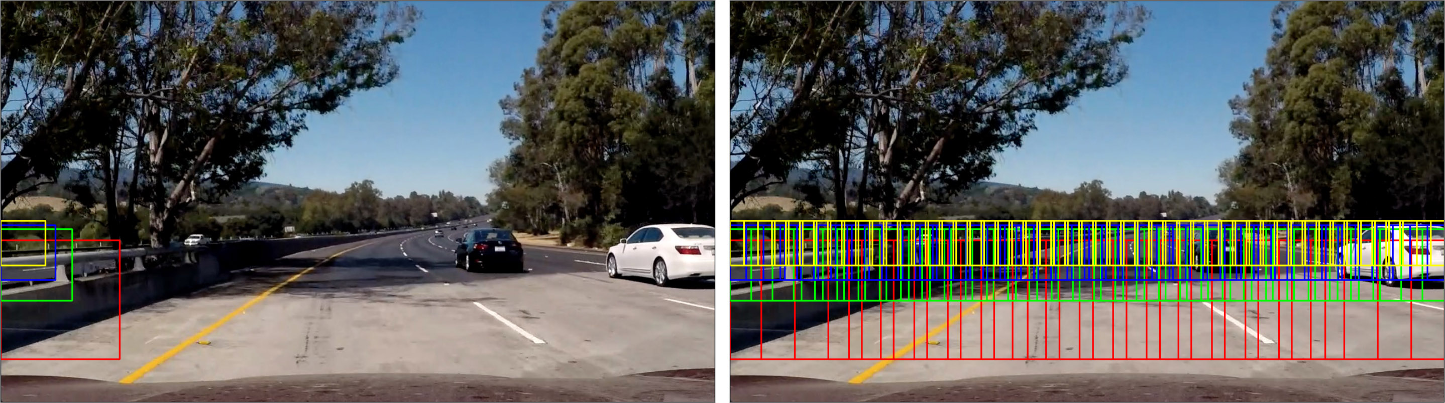
Window size varies across scanning locations

Since frame segments must be of various size, and we eventually need to use 64×64 regions as a classifier input, I decided to simply scale the frame to various sizes and then scan them with a 64×64 window. This can be roughly encoded as follows.

# Scan with 64×64 window across 8 differently scaled images, ranging from 30% to 80% of the original frame size. 
for (scale, y) in zip(np.linspace(.3, .8, 4), np.logspace(.6, .55, 4)):
    # Scale the original frame
    scaled = resize(image, (image.shape[0] * scale, image.shape[1] * scale, image.shape[2]))
    # Prepare a feature extractor
    extractor = FeatureExtractor(scaled)
    (h, w, d) = scaled.shape
    s = 64 // 3
    # Target stride is no more than s (1/3 of the window size here), 
    # making sure windows are equally distributed along the frame width.
    for x in np.linspace(0, w - k, (w + s) // s):
        # Extract features for current window.
        features = extractor.feature_vector(x, h*y, 64)
        # Run features through a scaler and classifier and add window coordinates 
        # to `detections` if classified as containing a vehicle
        ...

Merging multiple detections

As there are multiple detections on different scales and overlapping windows, we need to merge nearby detections. In order to do that we calculate a heatmap of intersecting regions that were classified as containing vehicles.

heatmap = np.zeros((image.shape[0], image.shape[1]))
# Add heat to each box in box list
for c in detections:
    # Assuming each set of coordinates takes the form (x1, y1, x2, y2)
    heatmap[c[1]:c[3], c[0]:c[2]] += 1
# Apply threshold to help remove false positives
heatmap[heatmap < threshold] = 0

Then we use label() function from scipy.ndimage.measurements module to detect individual groups of detections, and calculate a bounding rect for each of them.

groups = label(heatmap)
detections = np.empty([0, 4])
# Iterate through all labeled groups
for group in range(1, groups[1] + 1):
    # Find pixels belonging to the same group
    nonzero = (groups[0] == group).nonzero()
    detections = np.append(
        detections,
        [[np.min(nonzero[1]), np.min(nonzero[0]), np.max(nonzero[1]), np.max(nonzero[0])]],
        axis=0
    )

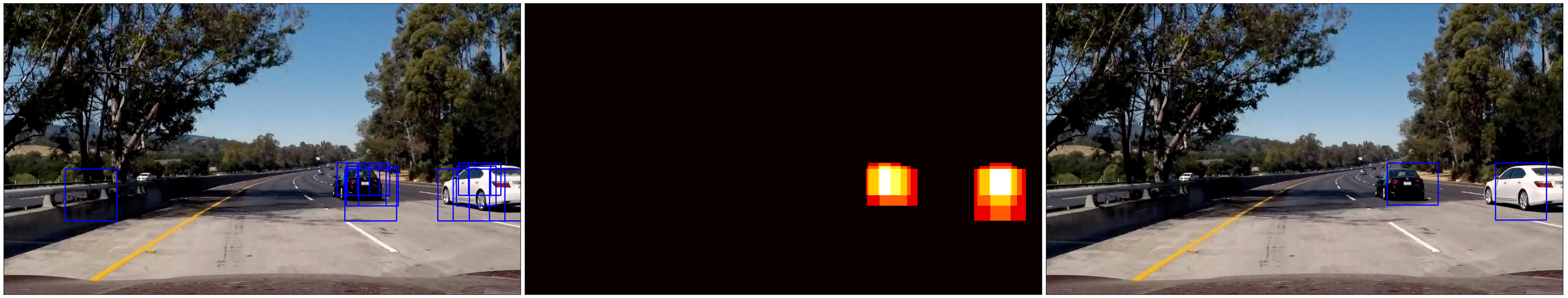
Merging detections with a heat map

Sequence of frames

Working with video allowes us to use a couple of additional constraints, in a sense that we expect it to be a stream of consecutive frames. In order to eliminate false positives I, again, use deque collection type in order to accumulate detections over last N frames instead of classifying each frame individually. And before returning a final set of detected regions I run those accumulated detections through the heatmap merging process once again, but with a higher detection threshold.

detections_history = deque(maxlen=20)

def process(frame):
    ...
    # Scan frame with windows through a classifier
    ...
    # Merge detections
    ...
    # Add merged detections to history
    detections_history.append(detections)

def heatmap_merge(detections, threshold):
    # Calculate heatmap for detections
    ...
    # Apply threshold
    ...
    # Merge detections with `label() 
    ...
    # Calculate bounding rects
    ...

def detections():
    return heatmap_merge(
        np.concatenate(np.array(detections_history)),
        threshold=min(len(detections_history), 15)
    )

This approach proved iself to work reasonably well on the source video, you can check out the full annotated video here. There is the current frame heat map in the top right corner — you may notice quite a few false positives, but most of them are eliminated by merging detections over the last N consecutive frames.

Sample of the annotated project video

For implementation details check VehicleTracker class in vehicletracker/tracker.py.

Results

This clearly is a very naive way of detecting and tracking road features, and wouldn’t be used in real world application as-is, since it is likely to fail in too many scenarios:

• Going up or down the hill.
• Changing weather conditions.
• Worn out lane markings.
• Obstruction by other vehicles or vehicles obstructing each other.
• Vehicles and vehicle positions different from those classifier was trained on.
• …

Not to mention it is painfully slow and would not run in real time without substantial optimisations. Nevertheless this project is a good representation of what can be done by simply inspecting pixel values’ gradients and color spaces. It shows that even with these limited tools we can extract a lot of useful information from an image, and that this information can potentially be used as a feature input to more sophisticated algorithms.

Follow @alexstaravoitau Star Fork Download