
I’m assuming you already know a fair bit about neural networks and regularization, as I won’t go into too much detail about their background and how they work. I am using Keras with TensorFlow backend as a ML framework and a couple of dependancies like numpy, pandas and scikit-image. You may want to check out code of the final solution I am describing in this tutorial, however keep in mind that if you would like to follow along, you may as well need a machine with a CUDA-capable GPU.
Training a model to drive a car in a simulator is one of the assignments in Udacity Self-Driving Car Nanodegree program, however the concepts described here should be easy to follow even without that context.
Dataset
The provided driving simulator had two different tracks. One of them was used for collecting training data, and the other one — never seen by the model — as a substitute for test set.
Data collection
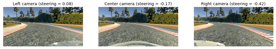
The driving simulator would save frames from three front-facing “cameras”, recording data from the car’s point of view; as well as various driving statistics like throttle, speed and steering angle. We are going to use camera data as model input and expect it to predict the steering angle in the [-1, 1] range.
I have collected a dataset containing approximately 1 hour worth of driving data around one of the given tracks. This would contain both driving in “smooth” mode (staying right in the middle of the road for the whole lap), and “recovery” mode (letting the car drive off center and then interfering to steer it back in the middle).
Balancing dataset
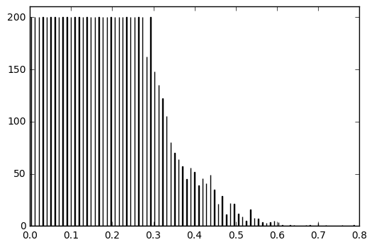
Just as one would expect, resulting dataset was extremely unbalanced and had a lot of examples with steering angles close to 0 (e.g. when the wheel is “at rest” and not steering while driving in a straight line). So I applied a designated random sampling which ensured that the data is as balanced across steering angles as possible. This process included splitting steering angles into n bins and using at most 200 frames for each bin:
df = read_csv('data/driving_log.csv')

balanced = pd.DataFrame()   # Balanced dataset
bins = 1000                 # N of bins
bin_n = 200                 # N of examples to include in each bin (at most)

start = 0
for end in np.linspace(0, 1, num=bins):
    df_range = df[(np.absolute(df.steering) >= start) & (np.absolute(df.steering) < end)]
    range_n = min(bin_n, df_range.shape[0])
    balanced = pd.concat([balanced, df_range.sample(range_n)])
    start = end
balanced.to_csv('data/driving_log_balanced.csv', index=False)
Histogram of the resulting dataset looks fairly balanced across most “popular” steering angles.
 Dataset histogram
Please, mind that we are balancing dataset across absolute values, as by applying horizontal flip during augmentation we end up using both positive and negative steering angles for each frame.
Data augmentation
After balancing ~1 hour worth of driving data we ended up with 7,698 samples, which most likely wouldn’t be enough for the model to generalise well. However, as many pointed out, there a couple of augmentation tricks that should let you extend the dataset significantly:
- Left and right cameras. Along with each sample we receive frames from 3 camera positions: left, center and right. Although we are only going to use central camera while driving, we can still use left and right cameras data during training after applying steering angle correction, increasing number of examples by a factor of 3.
cameras = ['left', 'center', 'right']
steering_correction = [.25, 0., -.25]
camera = np.random.randint(len(cameras))
image = mpimg.imread(data[cameras[camera]].values[i])
angle = data.steering.values[i] + steering_correction[camera]
- Horizontal flip. For every batch we flip half of the frames horizontally and change the sign of the steering angle, thus yet increasing number of examples by a factor of 2.
flip_indices = random.sample(range(x.shape[0]), int(x.shape[0] / 2))
x[flip_indices] = x[flip_indices, :, ::-1, :]
y[flip_indices] = -y[flip_indices]
- Vertical shift. We cut out insignificant top and bottom portions of the image during preprocessing, and choosing the amount of frame to crop at random should increase the ability of the model to generalise.
top = int(random.uniform(.325, .425) * image.shape[0])
bottom = int(random.uniform(.075, .175) * image.shape[0])
image = image[top:-bottom, :]
- Random shadow. We add a random vertical “shadow” by decreasing brightness of a frame slice, hoping to make the model invariant to actual shadows on the road.
h, w = image.shape[0], image.shape[1]
[x1, x2] = np.random.choice(w, 2, replace=False)
k = h / (x2 - x1)
b = - k * x1
for i in range(h):
    c = int((i - b) / k)
    image[i, :c, :] = (image[i, :c, :] * .5).astype(np.int32)
We then preprocess each frame by cropping top and bottom of the image and resizing to a shape our model expects (32×128×3, RGB pixel intensities of a 32×128 image). The resizing operation also takes care of scaling pixel values to [0, 1].
image = skimage.transform.resize(image, (32, 128, 3))
To make a better sense of it, let’s consider an example of a single recorded sample that we turn into 16 training samples by using frames from all three cameras and applying aforementioned augmentation pipeline.
 Original frames
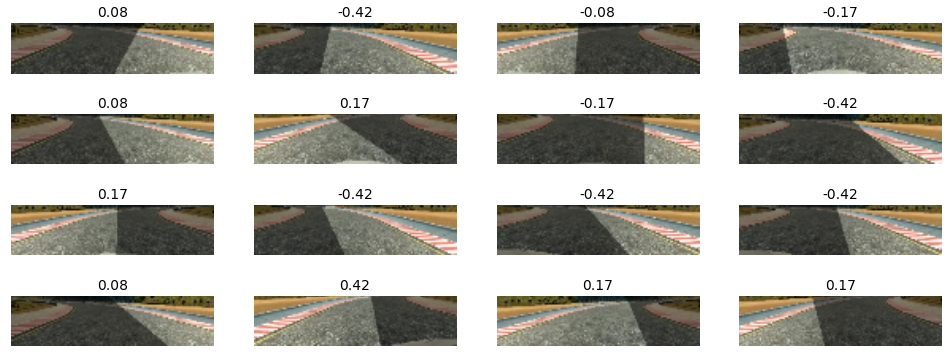 Augmented and preprocessed frames
Augmentation pipeline is applied in data.py using a Keras generator, which lets us do it in real-time on CPU while GPU is busy backpropagating!
Model
I started with the model described in Nvidia paper and kept simplifying and optimising it while making sure it performs well on both tracks. It was clear we wouldn’t need that complicated model, as the data we are working with is way simpler and much more constrained than the one Nvidia team had to deal with when running their model. Eventually I settled on a fairly simple architecture with 3 convolutional layers and 3 fully connected layers.
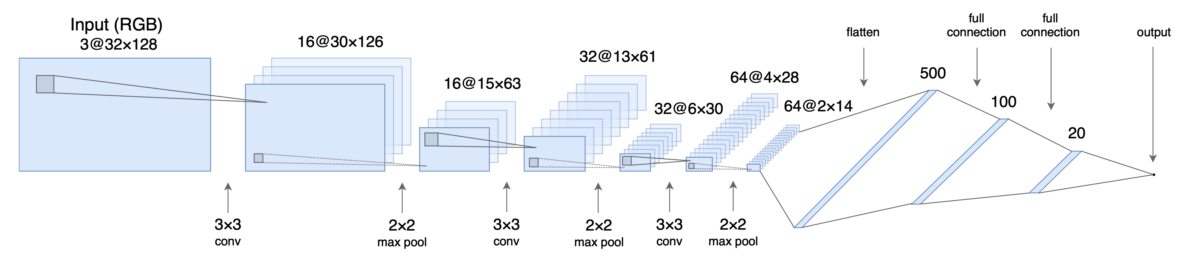
Model architecture
This model can be very briefly encoded with Keras.
from keras import models
from keras.layers import core, convolutional, pooling

model = models.Sequential()
model.add(convolutional.Convolution2D(16, 3, 3, input_shape=(32, 128, 3), activation='relu'))
model.add(pooling.MaxPooling2D(pool_size=(2, 2)))
model.add(convolutional.Convolution2D(32, 3, 3, activation='relu'))
model.add(pooling.MaxPooling2D(pool_size=(2, 2)))
model.add(convolutional.Convolution2D(64, 3, 3, activation='relu'))
model.add(pooling.MaxPooling2D(pool_size=(2, 2)))
model.add(core.Flatten())
model.add(core.Dense(500, activation='relu'))
model.add(core.Dense(100, activation='relu'))
model.add(core.Dense(20, activation='relu'))
model.add(core.Dense(1))
I added dropout on 2 out of 3 dense layers to prevent overfitting, and the model proved to generalise quite well. The model was trained using Adam optimiser with a learning rate = 1e-04 and mean squared error as a loss function. I used 20% of the training data for validation (which means that we only used 6,158 out of 7,698 examples for training), and the model seems to perform quite well after training for ~20 epochs — you can find the code related to training in model.py.
Results
The car manages to drive just fine on both tracks pretty much endlessly. It rarely goes off the middle of the road, this is what driving looks like on track 2 (previously unseen).
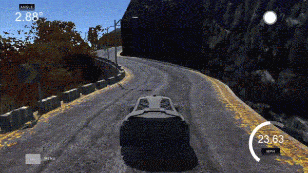 Driving autonomously on a previously unseen track
You can check out a longer highlights compilation video of the car driving itself on both tracks.
Clearly this is a very basic example of end-to-end learning for self-driving cars, nevertheless it should give a rough idea of what these models are capable of, even considering all limitations of training and validating solely on a virtual driving simulator.
Leave a Comment