I’m assuming you already know a fair bit about neural networks and regularization, as I won’t go into too much detail about their background and how they work. I am using TensorFlow as a ML framework and a couple of dependencies like numpy, matplotlib and scikit-image. In case you are not familiar with TensorFlow, make sure to check out my recent post about its core concepts.
If you would like to follow along, you may as well need a machine with a CUDA-capable GPU and all dependencies installed. Here is a Jupyter notebook with the final solution I am describing in this tutorial, presumably if you go through all the cells you should get the same results.
Dataset
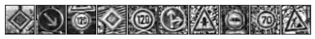
The German Traffic Sign Dataset consists of 39,209 32×32 px color images that we are supposed to use for training, and 12,630 images that we will use for testing. Each image is a photo of a traffic sign belonging to one of 43 classes, e.g. traffic sign types.
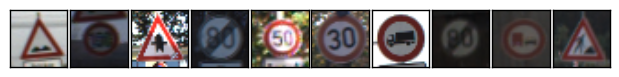 Random dataset sample
Each image is a 32×32×3 array of pixel intensities, represented as [0, 255] integer values in RGB color space. Class of each image is encoded as an integer in a 0 to 42 range. Let’s check if the training dataset is balanced across classes.
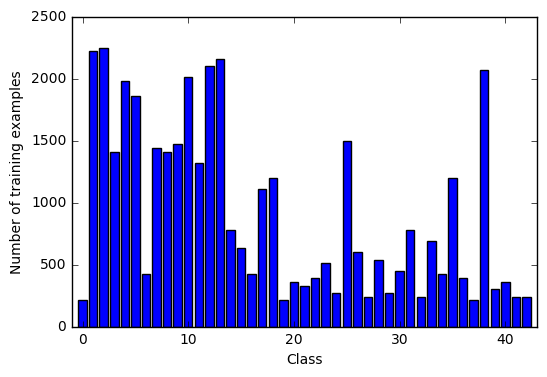 Dataset classes distribution
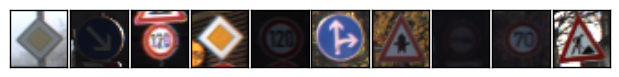
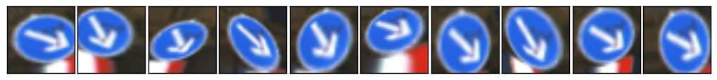
Apparently dataset is very unbalanced, and some classes are represented significantly better than the others. Let’s now plot a bunch of random images for various classes to see what we are working with.
 Yield
Yield
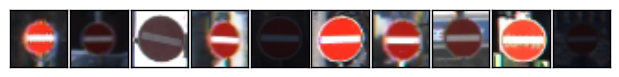 No entry
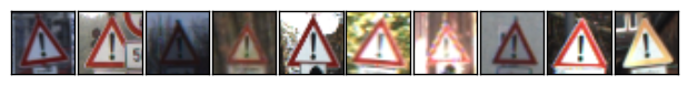 General caution
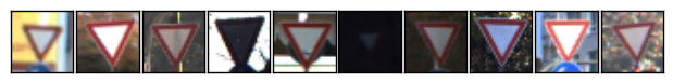
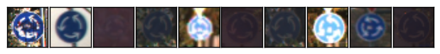 Roundabout mandatory
The images differ significantly in terms of contrast and brightness, so we will need to apply some kind of histogram equalization, this should noticeably improve feature extraction.
Preprocessing
The usual preprocessing in this case would include scaling of pixel values to [0, 1] (as currently they are in [0, 255] range), representing labels in a one-hot encoding and shuffling. Looking at the images, histogram equalization may be helpful as well. We will apply localized histogram equalization, as it seems to improve feature extraction even further in our case.
I will only use a single channel in my model, e.g. grayscale images instead of color ones. As Pierre Sermanet and Yann LeCun mentioned in their paper, using color channels didn’t seem to improve things a lot, so I will only take Y channel of the YCbCr representation of an image.
import numpy as np
from sklearn.utils import shuffle
from skimage import exposure

def preprocess_dataset(X, y = None):
    #Convert to grayscale, e.g. single Y channel
    X = 0.299 * X[:, :, :, 0] + 0.587 * X[:, :, :, 1] + 0.114 * X[:, :, :, 2]
    #Scale features to be in [0, 1]
    X = (X / 255.).astype(np.float32)

    # Apply localized histogram localization
    for i in range(X.shape[0]):
        X[i] = exposure.equalize_adapthist(X[i])

    if y is not None:
        # Convert to one-hot encoding. Convert back with `y = y.nonzero()[1]`
        y = np.eye(43)[y]
        # Shuffle the data
        X, y = shuffle(X, y)

    # Add a single grayscale channel
    X = X.reshape(X.shape + (1,))
    return X, y
This is what original and preprocessed images look like:
 Original
 Preprocessed
Augmentation
The amount of data we have is not sufficient for a model to generalise well. It is also fairly unbalanced, and some classes are represented to significantly lower extent than the others. But we will fix this with data augmentation!
Flipping
First, we are going to apply a couple of tricks to extend our data by flipping. You might have noticed that some traffic signs are invariant to horizontal and/or vertical flipping, which basically means that we can flip an image and it should still be classified as belonging to the same class.
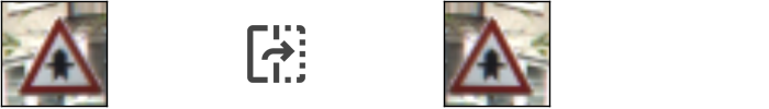
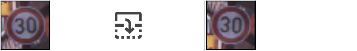
Some signs can be flipped either way — like Priority Road or No Entry signs.
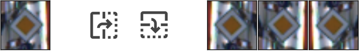
Other signs are 180° rotation invariant, and to rotate them 180° we will simply first flip them horizontally, and then vertically.
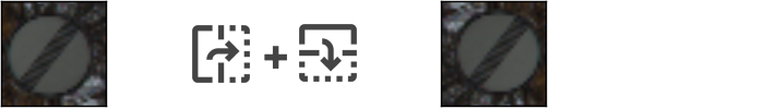
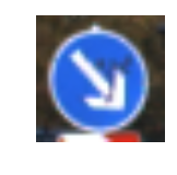
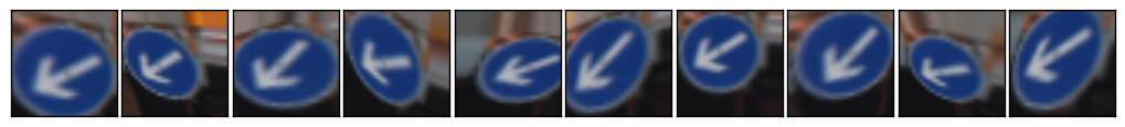
Finally there are signs that can be flipped, and should then be classified as a sign of some other class. This is still useful, as we can use data of these classes to extend their counterparts.
 Turn left Turn right
We are going to use this during augmentation. Let’s prepare a sign-flipping routine.
import numpy as np

def flip_extend(X, y):
    # Classes of signs that, when flipped horizontally, should still be classified as the same class
    self_flippable_horizontally = np.array([11, 12, 13, 15, 17, 18, 22, 26, 30, 35])
    # Classes of signs that, when flipped vertically, should still be classified as the same class
    self_flippable_vertically = np.array([1, 5, 12, 15, 17])
    # Classes of signs that, when flipped horizontally and then vertically, should still be classified as the same class
    self_flippable_both = np.array([32, 40])
    # Classes of signs that, when flipped horizontally, would still be meaningful, but should be classified as some other class
    cross_flippable = np.array([
        [19, 20],
        [33, 34],
        [36, 37],
        [38, 39],
        [20, 19],
        [34, 33],
        [37, 36],
        [39, 38],
    ])
    num_classes = 43

    X_extended = np.empty([0, X.shape[1], X.shape[2], X.shape[3]], dtype = X.dtype)
    y_extended = np.empty([0], dtype = y.dtype)

    for c in range(num_classes):
        # First copy existing data for this class
        X_extended = np.append(X_extended, X[y == c], axis = 0)
        # If we can flip images of this class horizontally and they would still belong to said class...
        if c in self_flippable_horizontally:
            # ...Copy their flipped versions into extended array.
            X_extended = np.append(X_extended, X[y == c][:, :, ::-1, :], axis = 0)
        # If we can flip images of this class horizontally and they would belong to other class...
        if c in cross_flippable[:, 0]:
            # ...Copy flipped images of that other class to the extended array.
            flip_class = cross_flippable[cross_flippable[:, 0] == c][0][1]
            X_extended = np.append(X_extended, X[y == flip_class][:, :, ::-1, :], axis = 0)
        # Fill labels for added images set to current class.
        y_extended = np.append(y_extended, np.full((X_extended.shape[0] - y_extended.shape[0]), c, dtype = int))

        # If we can flip images of this class vertically and they would still belong to said class...
        if c in self_flippable_vertically:
            # ...Copy their flipped versions into extended array.
            X_extended = np.append(X_extended, X_extended[y_extended == c][:, ::-1, :, :], axis = 0)
        # Fill labels for added images set to current class.
        y_extended = np.append(y_extended, np.full((X_extended.shape[0] - y_extended.shape[0]), c, dtype = int))

        # If we can flip images of this class horizontally AND vertically and they would still belong to said class...
        if c in self_flippable_both:
            # ...Copy their flipped versions into extended array.
            X_extended = np.append(X_extended, X_extended[y_extended == c][:, ::-1, ::-1, :], axis = 0)
        # Fill labels for added images set to current class.
        y_extended = np.append(y_extended, np.full((X_extended.shape[0] - y_extended.shape[0]), c, dtype = int))

    return (X_extended, y_extended)
This simple trick lets us extend original 39,209 training examples to 63,538, nice! And it cost us nothing in terms of data collection or computational resources.
Rotation and projection
However, it is still not enough, and we need to augment even further. After experimenting with adding random rotation, projection, blur, noize and gamma adjusting, I have used rotation and projection transformations in the pipeline. Projection transform seems to also take care of random shearing and scaling as we randomly position image corners in a [±delta, ±delta] range.
from skimage.transform import rotate
from skimage.transform import warp
from skimage.transform import ProjectiveTransform

def rotate(X, intensity):
    for i in range(X.shape[0])):
        delta = 30. * intensity # scale using augmentation intensity
        X[i] = rotate(X[i], random.uniform(-delta, delta), mode = 'edge')
    return X

def apply_projection_transform(X, intensity):
    image_size = X.shape[1]
    d = image_size * 0.3 * intensity
    for i in range(X.shape[0])):
        tl_top = random.uniform(-d, d)     # Top left corner, top margin
        tl_left = random.uniform(-d, d)    # Top left corner, left margin
        bl_bottom = random.uniform(-d, d)  # Bottom left corner, bottom margin
        bl_left = random.uniform(-d, d)    # Bottom left corner, left margin
        tr_top = random.uniform(-d, d)     # Top right corner, top margin
        tr_right = random.uniform(-d, d)   # Top right corner, right margin
        br_bottom = random.uniform(-d, d)  # Bottom right corner, bottom margin
        br_right = random.uniform(-d, d)   # Bottom right corner, right margin

        transform = ProjectiveTransform()
        transform.estimate(np.array((
                (tl_left, tl_top),
                (bl_left, image_size - bl_bottom),
                (image_size - br_right, image_size - br_bottom),
                (image_size - tr_right, tr_top)
            )), np.array((
                (0, 0),
                (0, image_size),
                (image_size, image_size),
                (image_size, 0)
            )))
        X[i] = warp(X[i], transform, output_shape=(image_size, image_size), order = 1, mode = 'edge')

    return X
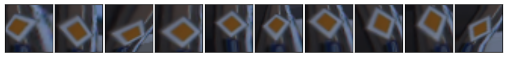
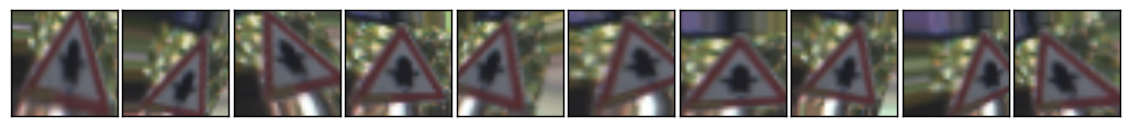
Please note that we use edge mode when applying our transformations, to ensure that we don’t have black box around warped image. Let’s check out what the images look like when we apply random augmentation with intensity = 0.75.
| Original | Augmented (intensity = 0.75) |
 |
 |
 |
 |
 |
 |
 |
 |
 |
 |
Model
Architecture
I decided to use a deep neural network classifier as a model, which was inspired by Daniel Nouri’s tutorial and aforementioned Pierre Sermanet / Yann LeCun paper. It is fairly simple and has 4 layers: 3 convolutional layers for feature extraction and one fully connected layer as a classifier.
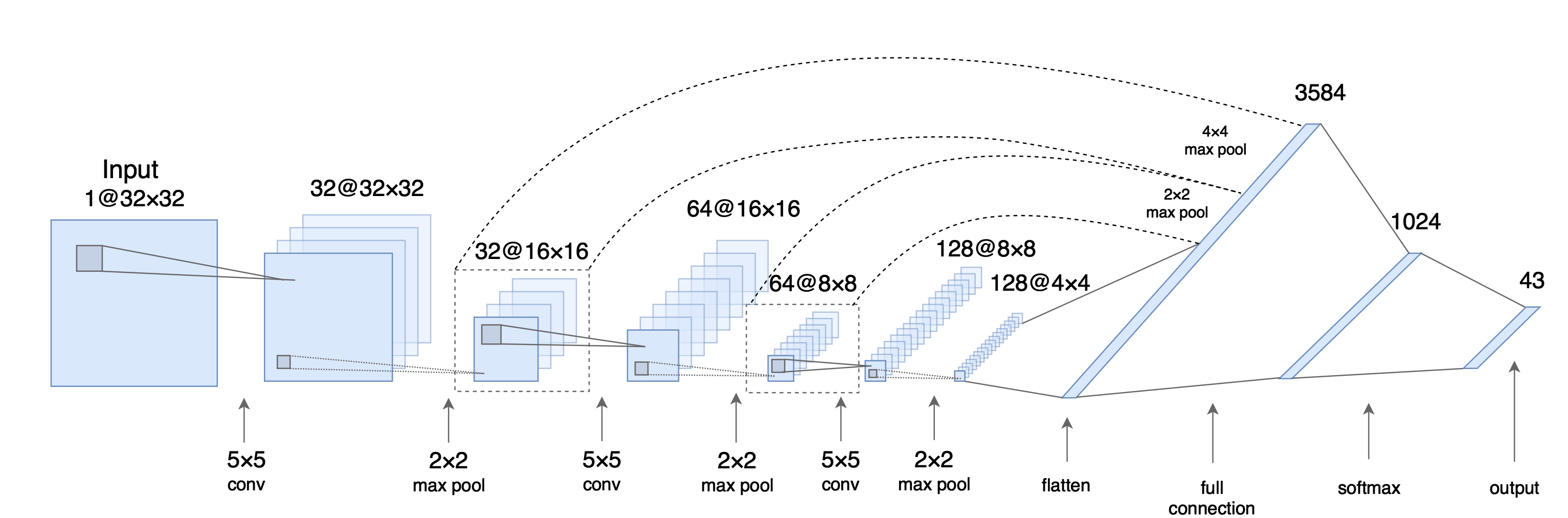
Model architecture
As opposed to usual strict feed-forward CNNs I use multi-scale features, which means that convolutional layers’ output is not only forwarded into subsequent layer, but is also branched off and fed into classifier (e.g. fully connected layer). Please mind that these branched off layers undergo additional max-pooling, so that all convolutions are proportionally subsampled before going into classifier.
Regularization
I use the following regularization techniques to minimize overfitting to training data:
- Dropout. Dropout is amazing and will drastically improve generalization of your model. Normally you may only want to apply dropout to fully connected layers, as shared weights in convolutional layers are good regularizers themselves. However, I did notice a slight improvement in performance when using a bit of dropout on convolutional layers, thus left it in, but kept it at minimum:
                Type           Size         keep_p      Dropout
 Layer 1        5x5 Conv       32           0.9         10% of neurons
 Layer 2        5x5 Conv       64           0.8         20% of neurons
 Layer 3        5x5 Conv       128          0.7         30% of neurons
 Layer 4        FC             1024         0.5         50% of neurons
-
L2 Regularization. I ended up using lambda = 0.0001 which seemed to perform best. Important point here is that L2 loss should only include weights of the fully connected layers, and normally it doesn’t include bias term. Intuition behind it being that bias term is not contributing to overfitting, as it is not adding any new degree of freedom to a model.
-
Early stopping. I use early stopping with a patience of 100 epochs to capture the last best-performing weights and roll back when model starts overfitting training data. I use validation set cross entropy loss as an early stopping metric, intuition behind using it instead of accuracy is that if your model is confident about its predictions it should generalize better.
Implementation
I find it helpful defining a structure holding hyperparameters I will be experimenting with and fine-tuning. It makes the process of tuning them easier, and even automate it in some cases.
from collections import namedtuple

Parameters = namedtuple('Parameters', [
        # Data parameters
        'num_classes', 'image_size',
        # Training parameters
        'batch_size', 'max_epochs', 'log_epoch', 'print_epoch',
        # Optimisations
        'learning_rate_decay', 'learning_rate',
        'l2_reg_enabled', 'l2_lambda',
        'early_stopping_enabled', 'early_stopping_patience',
        'resume_training',
        # Layers architecture
        'conv1_k', 'conv1_d', 'conv1_p',
        'conv2_k', 'conv2_d', 'conv2_p',
        'conv3_k', 'conv3_d', 'conv3_p',
        'fc4_size', 'fc4_p'
    ])
Let’s first declare a couple of helpful TensorFlow routines that implement individual types of layers.
import tensorflow as tf

def fully_connected(input, size):
    weights = tf.get_variable( 'weights',
        shape = [input.get_shape()[1], size],
        initializer = tf.contrib.layers.xavier_initializer()
      )
    biases = tf.get_variable( 'biases',
        shape = [size],
        initializer = tf.constant_initializer(0.0)
      )
    return tf.matmul(input, weights) + biases

def fully_connected_relu(input, size):
    return tf.nn.relu(fully_connected(input, size))

def conv_relu(input, kernel_size, depth):
    weights = tf.get_variable( 'weights',
        shape = [kernel_size, kernel_size, input.get_shape()[3], depth],
        initializer = tf.contrib.layers.xavier_initializer()
      )
    biases = tf.get_variable( 'biases',
        shape = [depth],
        initializer = tf.constant_initializer(0.0)
      )
    conv = tf.nn.conv2d(input, weights,
        strides = [1, 1, 1, 1], padding = 'SAME')
    return tf.nn.relu(conv + biases)

def pool(input, size):
    return tf.nn.max_pool(
        input,
        ksize = [1, size, size, 1],
        strides = [1, size, size, 1],
        padding = 'SAME'
    )
I am using Xavier initializer, which automatically determines the scale of initialization based on the layers’ dimensions, hence there are less parameter we need to experiment with.
We can now encode the model, getting most of variable scopes, which makes code easier to read and maintain. This method will perform a full model pass.
def model_pass(input, params, is_training):
    """
    Performs a full model pass.

    Parameters
    ----------
    input         : Tensor
                    Batch of examples.
    params        : Parameters
                    Structure (`namedtuple`) containing model parameters.
    is_training   : Tensor of type tf.bool
                    Flag indicating if we are training or not (e.g. whether to use dropout).

    Returns
    -------
    Tensor with predicted logits.
    """
    # Convolutions

    with tf.variable_scope('conv1'):
        conv1 = conv_relu(input, kernel_size = params.conv1_k, depth = params.conv1_d)
        pool1 = pool(conv1, size = 2)
        pool1 = tf.cond(is_training, lambda: tf.nn.dropout(pool1, keep_prob = params.conv1_p), lambda: pool1)
    with tf.variable_scope('conv2'):
        conv2 = conv_relu(pool1, kernel_size = params.conv2_k, depth = params.conv2_d)
        pool2 = pool(conv2, size = 2)
        pool2 = tf.cond(is_training, lambda: tf.nn.dropout(pool2, keep_prob = params.conv2_p), lambda: pool2)
    with tf.variable_scope('conv3'):
        conv3 = conv_relu(pool2, kernel_size = params.conv3_k, depth = params.conv3_d)
        pool3 = pool(conv3, size = 2)
        pool3 = tf.cond(is_training, lambda: tf.nn.dropout(pool3, keep_prob = params.conv3_p), lambda: pool3)

    # Fully connected

    # 1st stage output
    pool1 = pool(pool1, size = 4)
    shape = pool1.get_shape().as_list()
    pool1 = tf.reshape(pool1, [-1, shape[1] * shape[2] * shape[3]])

    # 2nd stage output
    pool2 = pool(pool2, size = 2)
    shape = pool2.get_shape().as_list()
    pool2 = tf.reshape(pool2, [-1, shape[1] * shape[2] * shape[3]])

    # 3rd stage output
    shape = pool3.get_shape().as_list()
    pool3 = tf.reshape(pool3, [-1, shape[1] * shape[2] * shape[3]])

    flattened = tf.concat(1, [pool1, pool2, pool3])

    with tf.variable_scope('fc4'):
        fc4 = fully_connected_relu(flattened, size = params.fc4_size)
        fc4 = tf.cond(is_training, lambda: tf.nn.dropout(fc4, keep_prob = params.fc4_p), lambda: fc4)
    with tf.variable_scope('out'):
        logits = fully_connected(fc4, size = params.num_classes)
    return logits
Note that we collect all branched off convolutional layers’ output, flatten and concatenate them before passing over to classifier.
If you have questions about TensorFlow implementation, make sure to check out my TensorFlow post about variable scopes, saving and restoring sessions, implementing dropout and other interesting things!
Training
I have generated two datasets for training my model using augmentation pipeline I mentioned earlier:
- Extended dataset. This dataset simply contains 20x more data than the original one — e.g. for each training example we generate 19 additional examples by jittering original image, with augmentation intensity = 0.75.
- Balanced dataset. This dataset is balanced across classes and has 20.000 examples for each class. These 20k contain original training dataset, as well as jittered images from the original training set (with augmentation intensity = 0.75) to complete number of examples for each class to 20.000 images.
Disclaimer: Training on extended dataset may not be the best idea, as some classes remain significantly less represented than the others there. Training a model with this dataset would make it biased towards predicting overrepresented classes. However, in our case we are trying to score highest accuracy on supplied test dataset, which (probably) follows the same classes distribution. So we are going to cheat a bit and use this extended dataset for pre-training — this has proven to make test set accuracy higher (although hardly makes a model perform better “in the field”!).
I then use 25% of these augmented datasets for validation while training in 2 stages:
- Stage 1: Pre-training. On the first stage I pre-train the model using extended training dataset with TensorFlow
AdamOptimizerand learning rate set to 0.001. It normally stops improving after ~180 epochs, which takes ~3.5 hours on my machine equipped with Nvidia GTX 1080 GPU. - Stage 2: Fine-tuning. I then train the model using a balanced dataset with a decreased learning rate of 0.0001.
These two training stages could easily get you past 99% accuracy on the test set. You can, however, improve model performance even further by re-generating balanced dataset with slightly decreased augmentation intensity and repeating 2nd fine-tuning stage a couple of times.
Visualization
As an illustration of what a trained neural network looks like, let’s plot weights of the first convolutional layer. First layer has dimensions of 5×5×1×32, which means that it consists of 32 5×5 filters — we can visualize them as 32 5×5 px grayscale images.
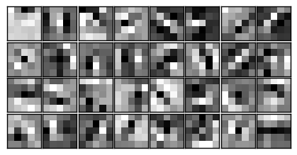 |
 |
| Raw | Interpolated |
We usually expect the first layer to contain filters that can detect very basic pixel patterns, like edges and lines. These basic filters are then used by subsequent layers as building bricks to construct detectors of more complicated patterns and figures.
Results
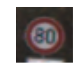
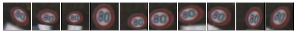
After a couple of fine-tuning training iterations this model scored 99.33% accuracy on the test set, which is not too bad. As there was a total of 12,630 images that we used for testing, apparently there are 85 examples that the model could not classify correctly — let’s take a look at those bad boys!
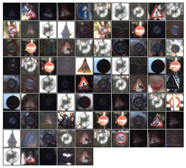 |
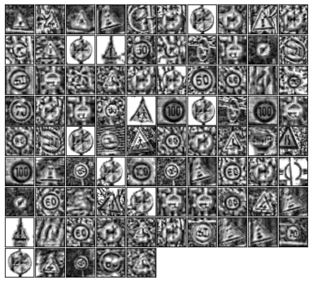 |
| Original | Preprocessed |
Signs on most of the images either have artefacts like shadows or obstructing objects. There are, however, a couple of signs that were simply underrepresented in the training set — training solely on balanced datasets could potentially eliminate this issue, and using some sort of color information could definitely help as well.
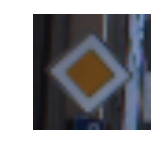
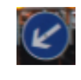
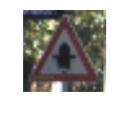
Finally, this model provides mildly interesting predictions for types of signs it wasn’t trained for.
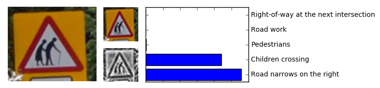 Predictions for a new type of sign
To clarify, this Elderly crossing sign was not among those 43 classes this model was trained for, yet what we see here is a reasonable assumption that it looks a lot like Road narrows on the right sign. Ironically, classifier’s second guess was that this Elderly crossing sign should be classified as Children crossing!
In conclusion, according to different sources human performance on a similar task varies from 98.3% to 98.8%, therefore this model seems to outperform an average human. Which, I believe, is the ultimate goal of machine learning!
Leave a Comment